Everything You Didn't Think You Needed to Know About Backsubstitution

Posted on Fri 03 January 2025 in miscellaneous

Introduction

The linear system, $\mathbf{Ax} = \mathbf{b}$ where $\mathbf{A}\in\mathbb{R}^{n\times n}$ and $\mathbf{x},\mathbf{b}\in\mathbb{R}^n$ can be solved in all manner of ways to yield some approximate solution, $\hat{\mathbf{x}}$. For the general matrix $\mathbf{A}$, the first algorithm one is exposed to is Gaussian Elimination, where $\mathbf{A}$ is first transformed into upper-triangular form through a series of row manipulations. Backsubstitution follows; each element of $\hat{\mathbf{x}}$ is solved for, starting from the final element, and subsequently used to solve for the next element of $\hat{\mathbf{x}}$. Backsubstitution will be the focus of this post.

This is perhaps best demonstrated through example. Consider

$$ \left[\begin{array}{ccc} A_{11} & A_{12} & A_{13} \\ 0 & A_{22} & A_{23} \\ 0 & 0 & A_{33} \end{array}\right] \left[\begin{array}{c} x_1 \\ x_2 \\ x_3 \end{array}\right] = \left[\begin{array}{c} b_1 \\ b_2 \\ b_3 \end{array}\right] \,. $$

$\hat{x}_3$ can be obtained trivially:

$$ A_{33} x_3 = b_3 \quad\rightarrow\quad \hat{x}_3 = \frac{1}{A_{33}}b_3 $$

Next, moving to $\hat{x}_2$,

$$ A_{22}x_2 + A_{23}x_3 = b_3 \quad\rightarrow\quad \hat{x}_2 = \frac{1}{A_{22}}\left[b_2 - A_{23}\hat{x}_3\right] $$

which can be solved since we have already solved for $\hat{x}_3$. Finally,

$$ A_{11}x_1 + A_{12}x_2 + A_{13}x_3 = b_1 \quad\rightarrow\quad \hat{x}_1 = \frac{1}{A_{11}}\left[ b_1 - A_{12}\hat{x}_2 - A_{13}\hat{x}_3\right] $$

This process can be generalised for any order matrix to take the form

$$ \hat{x}_k = \frac{1}{A_{kk}}\left[ b_k - \sum_{m=k+1}^n A_{km}\hat{x}_k\right] $$

Basic Implementation

Backsubstitution can be implemented in C++ as follows:

template<typename T>
void LinearSolver::solve(
    const SquareMatrix<T>& A, const std::vector<T>& b, std::vector<T>& x) 
{
    int order = static_cast<int>(x.size());
    for (int k=order - 1; k>=0; --k) {
        x[k] = b[k]
        for (int j=k; j<order; ++j) {
            x[k] -= A(k, j) * x[j];
        }
        x[k] /= A(k, k);
    }
}

Now, before you think me negligent, the above is written for clarity. If we want to make it performant, we'd have to remove the fact that A has the operator() overload to access elements, as well as the raw indexing into iterables. Rather, we should be using pointers or iterators and incrementing as we go, thereby removing overheads for things like function calls. Indeed, a compiler would refuse to vectorise the above because of the misdirection through overloaded operators. But as I said, we're more interested in clarity here.

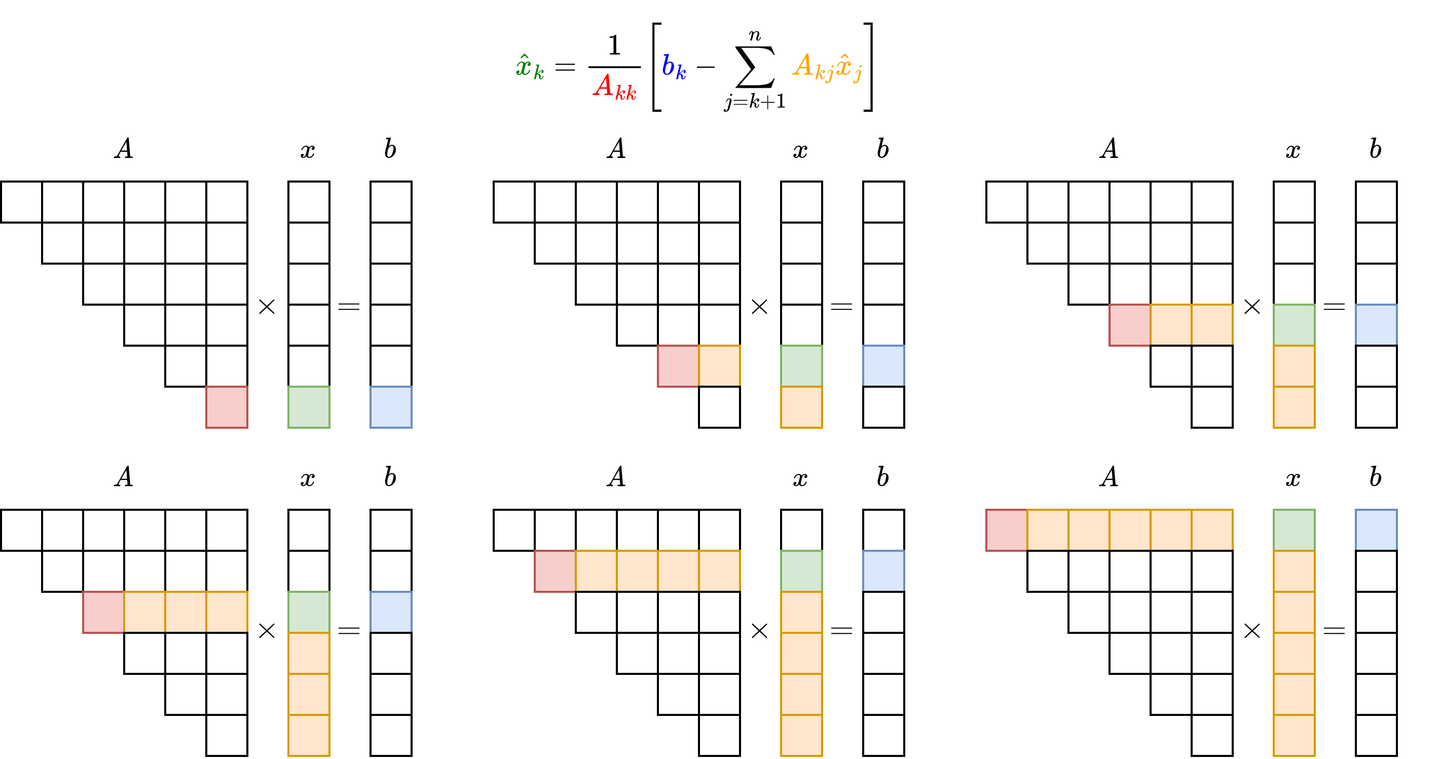
Let's explicitly walk through the algorithm in pictures. For a sixth order linear system, each outer loop iteration is shown as a frame in the image below:

Dependency Graph

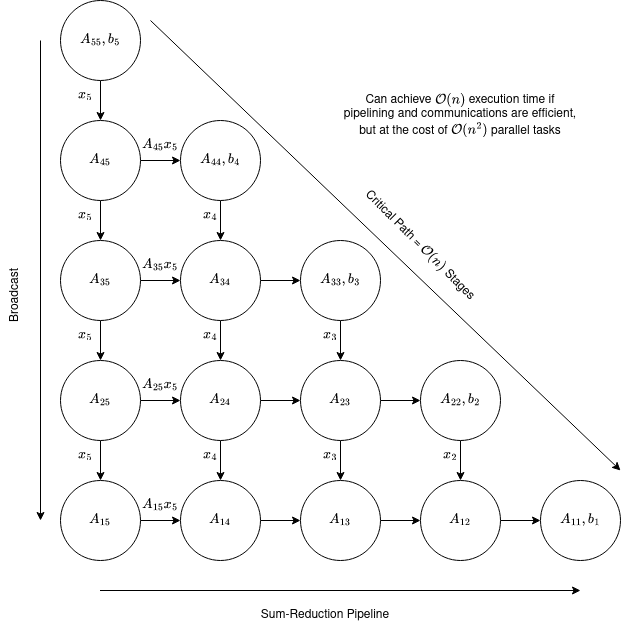
The best way to consider the scope for acceleration in an algorithm is to understand the dependencies therein. For backsubstitution, let's consider solving a fifth-order linear system. We can represent this as a directional graph, depicted below:

Each node in the graph corresponds to an operation; values are loaded from memory (shown by the quantities within the node) and edges show dependencies between nodes. Rows represent the sequence of operations required to compute $\hat{x}_{n-i+1}$ where $i$ enumerates the row. The top element of each column (on the diagonal) corresponds to the computation of $\hat{x}_{n-j+1}$ where $j$ enumerates the column; $\hat{x}_{n-j+1}$ is subsequently broadcast to all nodes beneath it in the column. In the following, we'll refer to nodes in the dependency graph by the pair $(i,j)$.

Let's consider a route through the graph. We start with the upper-left node which loads $A_{55}$ and $b_5$, then computes $\hat{x}_5$. Now, consider the expression for $\hat{x}_4$:

$$ \hat{x}_4 = \frac{1}{A_{44}}\left[ b_4 - A_{45}\hat{x}_5\right] \,. $$

First of all we take $\hat{x}_5$ from $(1,1)$ and multiply if with $A_{45}$ as suggested by $(2,1)$. This product can be passed onto $(2,2)$ which is free to compute $\hat{x}_4$ after loading $A_{44}$ and $b_4$.

Note that $(3,1)$ requires only $\hat{x}_5$, and consequently the product $A_{35}\hat{x}_5$ can be formed at the same time as $A_{45}\hat{x}_5$, so the calculation for $\hat{x}_3$ can begin concurrently with the calculation for $\hat{x}_4$, and by extension $\hat{x}_2$ and $\hat{x}_1$.

The dependency graph gives us a bit of insight in how we can attempt to implement backsubstitution. We can either move down an entire column before moving onto the next, or move across an entire row before moving onto the next. In the following, we'll write in C-like pseudocode. Let's take iterating across a row first, which we'll refer to as row-first:

x[:] = b[:];
for (int irow=n-1; irow>=0; --irow) {
    for (int icol=irow+1; icol<irow; ++icol) {
        x[irow] -= A(irow, icol) * x[icol];
    }
    x[irow] /= A(irow, irow);
}

Here, for each iteration of the outer loop, we do all the computation associated with calculating a single element of $\hat{\mathbf{x}}$ at a time, and end by outputting that element. Access to $\mathbf{A}$ is row-wise, hence a row-major ordering of the matrix is optimal for a memory access pattern, giving good spatial locality.

How about iterating down a column first?

x[:] = b[:];
for (int icol=n-1; icol>=0; --icol) {
    x[icol] /= A(icol, icol);
    for (int irow=0; irow<icol; ++irow) {
        x[irow] -= A(irow, icol) * x[icol];
    }
}

We'll refer to this implementation as column-first. The structure looks deceptively similar to the row-first implementation, but this is actually fundamentally different. On each outer-loop iteration, we begin by forming an element of $\hat{\mathbf{x}}$, and subsequently multiply the entire column of $\mathbf{A}$ by that element. In this way, we're adding a component to each of the sum-reduction pipelines per outer-loop iteration. Access to $\mathbf{A}$ is column-wise, hence a column-major ordering of the matrix is optimal for memory access pattern.

With all of this in mind, we can move onto attempting to accelerate backsubstitution.

Acceleration Strategies

The dependency graph shows us that the critical path of the algorithm is the route through the diagonals, which is $\mathcal{O}(n)$. Since there are $\mathcal{O}(n^2)$ nodes within the graph, if we were to devote a parallel process to each node, assuming no communications overhead, we could expect an $\mathcal{O}(n)$ runtime.

Clearly this isn't a particularly efficient use of resources, and hence we seek to agglomerate fine-grained tasks to run on a single parallel resource while approaching the speedup that's dictated by the algorithm's critical path length. Since we have two for-loops in our algorithm, there are (at least) two targets for parallelisation; the inner and outer loops. However, for the outer loop, there's a carried dependence between loop iterations; $\hat{x}_k$ depends on $\hat{x}_{k+1}$ that's computed the iteration before. Hence our ability to parallelise over this loop is restricted.

In the following, we'll first detail parallelism that can be leveraged on a single node, that is, SIMD parallelism. The rest of this section is then devoted to deploying backsubstitution in a parallel environment, whether that be with multithreading or multiprocessing. For the parallel environment discussion, we'll refer to a parallel unit as a "process", and discuss operations such as "broadcasting" which are strictly multiprocessing nomenclature. The reader should keep in mind that the discussion is equally valid for multithreading, but substituting "process" for "thread" and send/ receive operations for mutex-based counterparts.

SIMD

As we've already mentioned, there's no scope to parallelise the outermost loop in either the row-first or column-first orderings. As such, we'll focus on the innermost loop.

Let's take our row-first ordering. Each element in the sum-reduction pipeline requires a multiplication, so it seems as if we have an obvious target here. However, the subsequent reduction is a little more problematic; horizontal addition across a vector register isn't really a "proper" SIMD instruction, and typically requires some composite involving permutations and multiple vector additions. Even in those architectures which support horizontal additions, the order of reduction will be different from the serial code -- since floating point operations are no associative, this means there'll be some discrepancy between vectorised and serial implementations which may be problematic for some developers. Hence, pursuing this strategy for SIMD may be more painful than it's worth.

The column-first ordering, however, is a little more intriguing; we don't have to actually do any reduction across a vector register here; the reduction happens naturally as we accumulate to $\hat{\mathbf{x}}$ on each column.

We do, however, need to be a little careful here since the number of elements in the column we're working with won't always be some multiple of the vector width. As such, we either need to pad our arrays with zeros so that we don't access some forbidden or incorrect bit of memory when loading a vector register, or add some additional logic to our loops that handles edge elements. The second strategy is certainly more scalable; if the order of the linear system is large, then the number of padding elements will be enormous, hence a drain on memory capacity, not to mention bandwidth from loading zeroes.

As such, let's try to handle the edge elements appropriately:

constexpr std::size_t vec_width = 8;

x[:] = b[:];

for (int icol=n-1; icol>=0; --icol) {

    x[icol] /= A(icol, icol);

    const int num_vecs = icol / vec_width;
    const int edge_start = num_vecs * vec_width;

    for (int irow=0; irow<num_vecs; ++irow) {
        const int offset = irow * vec_width;
#pragma omp simd
        for (std::size_t ivec=0; ivec<vec_width; ++ivec) {
            x[offset+ivec] -= A(offset + ivec,icol) * x[icol];
        }
    }

    for (int irow=edge_start; irow<icol; ++irow) {
        x[irow] -= A(irow, icol) * x[icol];
    }
}

We've used OpenMP to be explicit in what we think should be vectorised; in reality, the compiler would likely identify this without our intervention. It's worth noting that there are certain architectures which do not require explicit edge handling in this way. ARM's SVE instruction set is "predicate-driven"; a predicate register is associated with each vector register, with the instruction only applied to those elements that the predicate permits.

Row Agglomeration

In this section, we'll discuss how we might deploy the "row-first" ordering in a parallel environment. In other words, let $k=n-i+1$; the $i^{th}$ parallel process computes the sum-reduction

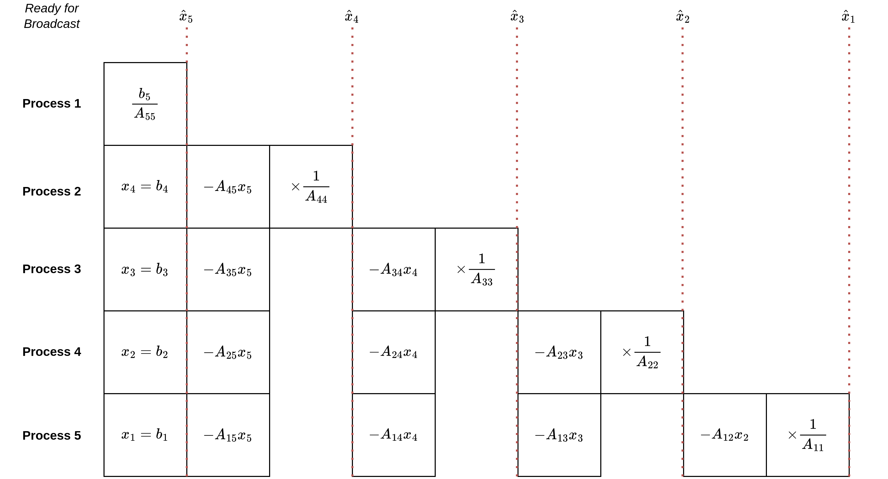
$$ \hat{x}_k = \frac{1}{A_{kk}}\left[ b_k - \sum_{j=0}^{k-1}A_{kj}\hat{x}_j\right] $$

and subsequently broadcasts $\hat{x}_k$ to all other processes $k^\prime > k$. The communications requirements for this strategy are $\mathcal{O}(n)$ broadcasts which can be temporally interleaved (i.e. multiple processes don't need to broadcast at the same time), hence there should be no contention for the communications channel. One can depict the rudimentary time/resource graph below:

The horizontal axis is discretised into timesteps, and for the sake of simplicity, the time taken for each arithmetic operation is equal. Furthermore, communications are instantaneous. These are clearly all incorrect, but are considered as such because it allows us to schedule the algorithm purely on data dependencies alone.

At the first time increment, we're able to compute $\hat{x}_5 = b_5 / A_{55}$. This value is subsequently broadcast to all other processes, $i=2,...,5$, which are consequently able to compute the contribution of $\hat{x}_5$ to their own solution elements, $A_{k,5}\hat{x}_5$. Since $\hat{x}_4$ depends only on $\hat{x}_5$, we're able to compute $\hat{x}_4$ during the next time increment and broadcast this to all other processes. This continues until $\hat{x}_1$ has been computed, at which point the algorithm terminates.

The time taken for this strategy is dictated by the length of the pipeline used to compute $\hat{x}_1$, which is clearly $\mathcal{O}(n)$. However, this would also require $\mathcal{O}(n)$ parallel processes, which is clearly excessive when $n$ is large. Furthermore, lower order processes will be idle for the vast majority of the runtime; the process that computes $\hat{x}_n$ performs a single division and does no more! As such, the implementation as we've detailed it is horribly inefficient.

Cyclic Row Agglomeration

However, all is not lost; the fact that lower order processes are idle for the majority of the runtime offers an opportunity since we can distribute work to them once they're done. If we have $N < n$ parallel processes available to us, then we can cyclically assign the computation of $\hat{x}_k$. Denote the cyclic index $\kappa = 1 + (n - k)\hphantom{\prime}\mathrm{mod}\hphantom{\prime}N$, then process $i$ will be given $\hat{x}_{\kappa}$. Let's modify our above example so that $N = 3$ and $n = 6$:

In the above, we've coloured in red those nodes that have been cyclically assigned to a process after its initial computation is done. We see that process 1 begins by computing and broadcasting $\hat{x}_6$, but can then immediately commence calculating $\hat{x}_3$ using $\hat{x}_6$. Similarly, process 2 begins by receiving $\hat{x}_6$ and subsequently computes $\hat{x}_5$. Once this is done though, it can immediately start proessing $\hat{x}_2$, and so on.

However, we note that the number of time increments has increased here relative to when $N = n$. The issue is that the process responsible for computing $\hat{x}_1$ has a runtime that controls the overall runtime of the computation. Since the process assigned to $\hat{x}_1$ is occupied when $N = n$ for virtually the entire runtime, adding more work onto that process clearly increases the runtime by some amount. However, this means that we can parallelise backsubstitution over arbitrary $N$ processes and obtain some $\mathcal{O}(N)$ speedup.

Column Agglomeration

In this section, we'll discuss how we might deploy the "column-first" ordering in a parallel environment. Each process is effectively in charge of performing one stage of each sum-reduction pipeline, perhaps something of a bizarre-sounding strategy, but let's take a look.

Now, once $\hat{x}_n$ is evaluated, it is used to compute the products $A_{1,n}\hat{x}_n,A_{2,n}\hat{x}_n,...,A_{n-1,n}$, i.e. multiplying $\hat{x}_n$ by the column $\mathbf{A}_{:,n}$. These correspond to a single term in the accumulation for each column's element of $\hat{\mathbf{x}}$. Let's introduce a new nomenclature for partial sums,

$$ S_k^j = -\sum_{\ell=0}^{j-1} A_{k,n-\ell}\hat{x}_{n-\ell} $$

where $k$ denotes the sum-reduction pipeline for $\hat{x}_k$, and $j$ the number of terms that have been accumulated into the reduction. Note also the recursion,

$$ S_k^{j+1} = S_k^j - A_{k,n-j}\hat{x}_{n-j} $$

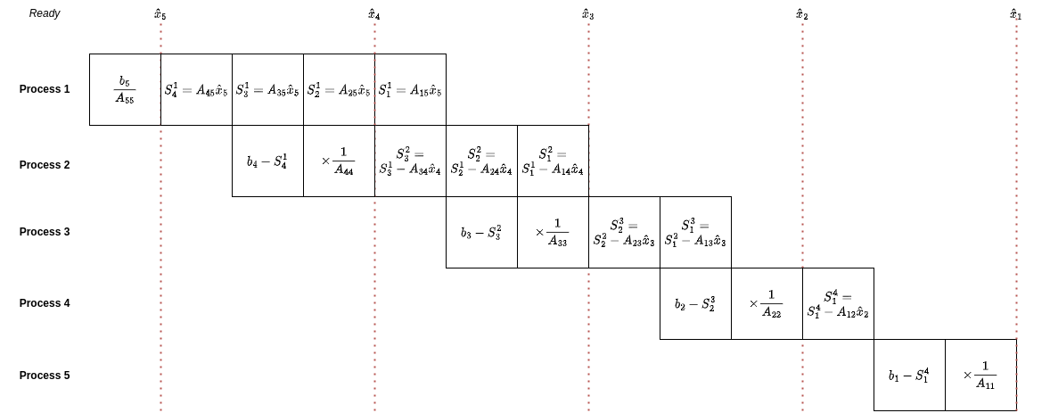
Armed with our new notation, let's draw the time/resource graph for column agglomeration:

As soon as $\hat{\mathbf{x}}_k$ has been computed, it is immediately multiplied by the column $\mathbf{A}_{:,k}$ and accumulated into the $S_k^j$ partial sums. Once $S_{k-1}^j$ has been computed, it can be sent to the process that's dedicated to computing $\hat{x}_{k-1}$, which is then able to compute the $S_{k-1:n}^{j+1}$.

We see then that the communication cost here is $\mathcal{O}(n^2)$; recall that the row-first ordering required $\mathcal{O}(n)$ broadcasts, and hence has the same communication cost. One might find it appealing to compute $\hat{x}_k$, compute all the $S_k^j$ and package these into a single message to be sent to the next process yielding $\mathcal{O}(n)$ communication overhead. However, notice that this is just the serial implementation, with the added complexity of starting the next portion of the algorithm on another thread, rendering this strategy fruitless.

We can, of course, perform cyclic column agglomeration much as we did in the previous section for row agglomeration; in our time/resource graph, we see that process 1 is idle when process 3 begins, so clearly there's the same scope to perform column agglomeration using $N < n$ processes as with row agglomeration.

Validation

Error Metrics

So now we have an implementation, we need to verify whether the solution we get out of the other end is correct or not. In other words, we want $\hat{\mathbf{x}} - \mathbf{x} \approx \mathbf{0}$. But note the approximation; how good is good enough? Is there some bound we can expect to attain based on the limitations of floating point arithmetic or even some features of the system?

We should begin by qualifying the metric we're to use in validating our solution. First and foremost, we're interested in relative errors, e.g. $\lVert\mathbf{x} - \hat{\mathbf{x}}\rVert / \lVert\mathbf{x}\rVert$. The choice of norm isn't enormously important here. Note that division by the norm of the true solution makes the error relative; this makes the metric more stable. If we're dealing with $\lVert\mathbf{x}\rVert \approx 10^3$, then $\lVert\mathbf{x} - \hat{\mathbf{x}}\rVert\approx 10^{-3}$ isn't as important as when $\lVert\mathbf{x}\rVert\approx 10^{-3}$. Hence making errors relative places into context, so to speak, the error that's been obtained.

Now, of course we don't know what $\hat{\mathbf{x}}$ is a priori, so how do we know what the error we've obtained is? We can use the residual:

$$ \mathbf{r} = \mathbf{b} - \mathbf{A}\hat{\mathbf{x}} $$

which presents us with an elementwise measure of how well $\mathbf{\hat{x}}$ solves the linear system. The relative residual is then $\rho(\hat{\mathbf{x}}) = \lVert\mathbf{r}\rVert / \lVert\mathbf{b}\rVert$. Notice that

\begin{align} \mathbf{A}^{-1}\mathbf{r} &= \mathbf{A}^{-1}\mathbf{b} - \mathbf{A}^{-1}\mathbf{A}\hat{\mathbf{x}}\\ &= \mathbf{A}^{-1}\mathbf{b} - \mathbf{A}^{-1}\mathbf{A}\hat{\mathbf{x}}\\ &= \mathbf{x} - \hat{\mathbf{x}} \end{align}

Now, dividing through by $\lVert\mathbf{x}\rVert$ to yield the residual error on the RHS, and recalling the triangle inequality for norms, i.e. $\lVert\mathbf{AB}\rVert \leq \lVert\mathbf{A}\rVert\lVert\mathbf{B}\rVert$,

\begin{align} \frac{\lVert\mathbf{x} - \hat{\mathbf{x}}\rVert}{\lVert\mathbf{x}\rVert} &= \frac{\lVert\mathbf{A}^{-1}\mathbf{r}\rVert}{\lVert\mathbf{x}\rVert} \leq \frac{\lVert\mathbf{A}^{-1}\rVert\lVert\mathbf{r}\rVert}{\lVert\mathbf{x}\rVert} \\ &\leq \frac{\lVert\mathbf{A}\rVert}{\lVert\mathbf{A}\rVert}\frac{\lVert\mathbf{A}^{-1}\rVert\lVert\mathbf{r}\rVert}{\lVert\mathbf{x}\rVert} =\kappa(\mathbf{A})\frac{\lVert\mathbf{r}\rVert}{\lVert\mathbf{b}\rVert} \\ &\leq \kappa(\mathbf{A})\rho(\hat{\mathbf{x}}) \end{align}

where $\kappa(\mathbf{A})$ is the condition number of the matrix $\mathbf{A}$. Thus, the relative error in $\mathbf{x}$ is bounded by a multiple of the relative residual, or the error in $\mathbf{b}$. The condition number measures the sensitivity of a linear system to being solved on a computer in the presence of inaccurate values. For instance, if the relative residual is $10^{-6}\%$ but $\kappa = 10^5$, we'd have an error of up to $10\%$ in the relative error.

What can we expect from the relative residual? Well, assuming the relative residual is non-zero, the smallest difference between $\mathbf{x}$ and $\hat{\mathbf{x}}$ would be the machine epsilon since some rounding error has taken place. Assuming $\lVert\mathbf{x}\rVert$ is of the order of unity, then the relative residual is of the order of the machine epsilon (clearly this isn't necessarily the case -- $\lVert\mathbf{x}\rVert$ could be enormous or miniscule, but we're choosing best case scenario here). $\mathbf{A}$ will then set how far the solution can deviate from its actual value to yield the associated relative residual.

Error Analysis

Backsubstitution incorporates a few different arithmetic operations, each of which brings in some error from rounding or representation error. Let's look at these one-at-a-time. First on our list is the summation,

$$ s_k = \sum_{j=k+1}^n A_{kj}\hat{x}_j $$

This is nothing more than a dot product between part of a row of $\mathbf{A}$ and part of $\hat{\mathbf{x}}$. We can write the floating point result from a multiplication using first-order perturbation theory, $\hat{z} = xy(1+\pi)$, and similarly for an addition, $\hat{z} = (x + y)(1 + \sigma)$. Let's consider the first term in our dot product -- we'll change the summation index bounds to $j=1,...,n$ for the sake of making notation cleaner. Then,

$$ \hat{s}_1 = A_{k,1}\hat{x}_1(1 + \pi_1) $$

Now, adding this with the next term in sequence,

$$ \hat{s}_2 = (A_{k,1}\hat{x}_1(1 + \pi_1) + A_{k,2}\hat{x}_{2}(1 + \pi_2))(1 + \sigma_1) $$

A third term will help us to generalise:

\begin{align} \hat{s}_3 &= ((A_{k,1}\hat{x}_1(1 + \pi_1) + A_{k,2}\hat{x}_{2}(1 + \pi_2))(1 + \sigma_1) + A_{k,3}\hat{x}_{3}(1 + \pi_3))(1 + \sigma_2) \\ &= A_{k,1}\hat{x}_1(1 + \pi_1)(1 + \sigma_1)(1 + \sigma_2) + A_{k,2}\hat{x}_2(1 + \pi_2)(1 + \sigma_1)(1 + \sigma_2) + A_{k,3}\hat{x}_3(1 + \pi_3)(1 + \sigma_2) \end{align}

A veritable mess. But now we'll omit any cross terms involving $\pi$ and $\sigma$, since if these are both of the order of the machine epsilon, they're inconsequential to our analysis:

$$ \hat{s}_3 = A_{k,1}\hat{x}_1(1 + \pi_1 + \sigma_1 + \sigma_2) + A_{k,2}\hat{x}_2(1 + \pi_2 + \sigma_1 + \sigma_2) + A_{k,3}\hat{x}_3(1 + \pi_3 + \sigma_2) + \mathcal{O}(\epsilon^2) $$

The emerging pattern resembles:

$$ \hat{s}_k \approx \sum_{i=1}^k A_{ik}\hat{x}_k(1 + (k-i)\delta) $$

where we've replaced $\sigma$ and $\pi$ with the generic $\delta$, and the prefactor of $(k-i)$ indicates that earlier terms in the sequence have more error contributions since they're added to more than later terms. In fact, we can bound the above

$$ \hat{s}_k \leq \sum_{i=i}^k A_{ik}\hat{x}_k(1 + k\delta) $$

Now, finding the explicit error between this and $s_k$,

\begin{align} \lVert s_k - \hat{s}_k\rVert &= \lVert \sum_{i=i}^k A_{ik}\hat{x}_k(1 + k\delta) - \sum_{i=i}^k A_{ik}\hat{x}_k\rVert\\ &= \lVert \sum_{i=i}^k A_{ik}\hat{x}_k k\delta\rVert \\ & \leq \sum_{i=1}^k\lVert A_{ik}\rVert \lVert x_{k}\rVert k \delta = \lVert A_{k,:}\rVert^\top \lVert x\rVert k \delta \end{align}

Refinement of the Solution

There is a mechanism by which, given some initial solution, $\hat{\mathbf{x}}_0$, we can reduce the residual until it meets some user-defined criterion. The following is iterative, and we'll use $m$ as the iteration index. Then:

Compute the residual, $\mathbf{r}_m = \mathbf{b} - \mathbf{A}\hat{\mathbf{x}}_m$
Solve the system for a correction, $\mathbf{c}_m$ which removes the residual, $\mathbf{A}\mathbf{c}_m = \mathbf{r}_m$
Add the correction to the previous solution, $\hat{\mathbf{x}}_{m+1} = \hat{\mathbf{x}}_m + \mathbf{c}_m$

Let's see why this works by looking at what the residual is after having corrected our initial guess:

$$ \mathbf{r}_{m+1} = \mathbf{b} - \mathbf{A}\hat{\mathbf{x}}_{m+1} = \mathbf{b} - \mathbf{A}\hat{\mathbf{x}}_m - \mathbf{A}\mathbf{c}_m $$

Multiplying through by $\mathbf{A}^{-1}$, we see that the LHS becomes $\mathbf{A}^{-1}\mathbf{r}_{m+1} = \mathbf{x} - \hat{\mathbf{x}}_{m+1}$ (the error at the next iteration) as shown in the previous section. Then

\begin{align} \mathbf{x} - \hat{\mathbf{x}}_{m+1} &= \mathbf{A}^{-1}\mathbf{b} - \mathbf{A}^{-1}\mathbf{A}\hat{\mathbf{x}}_m - \mathbf{A}^{-1}\mathbf{A}\mathbf{c}_m \\ &= \mathbf{x} - \hat{\mathbf{x}}_m - \mathbf{c}_m \end{align}

After a bit of rearrangement, we're left with

$$ \mathbf{x} - \hat{\mathbf{x}}_{m+1} = \mathbf{x} - \hat{\mathbf{x}}_{m} - \mathbf{c}_m $$

So our solution error at the next iteration is improved by $\mathbf{c}_m$.